Convex Optimization — Bounded Liquidity
Part III: Uniswap V3
The Uniswap V2 x*y=k invariant is simple to understand. Single V2 pools can easily be modeled as part of a convex optimization problem, and then vectorized for multi-pool optimizations.
However once you’ve understood Uniswap V2, your thoughts immediately drift to the critical question: “V3, wat do?”
Uniswap V3’s bounded liquidity model is harder to model because of the discontinuous nature, but understanding some concepts from the white paper enables us to model these pools as well.
Uniswap V3 — Key Concepts
Even if you’ve already read my complete Uniswap V3 series, I suggest reviewing the Pool Contract exploration.
The fundamental points you should understand are:
V3 pools primarily track liquidity and price
Price is expressed as a ratio of token1 per token0, or y/x
The price range is geometrically spaced using ticks, using 1 basis point (0.01%) intervals
Liquidity can be provided between any two ticks at an enforced minimum spacing
Inside a tick range, liquidity is constant — only the price varies through the action of swaps
The price varies in both directions until such time as it reaches a boundary where the in-range liquidity is changed
Fees collected by the pool are not redeposited as new liquidity, but rather held and given to the liquidity providers when they withdraw their positions
Achieve Capital Efficiency With This One Weird Trick
Here’s the secret about V3: it pretends to be one pool, but it’s really a bunch of V2 pools glued together using some clever accounting.
To understand this glib summary, you must understand the concept of virtual reserves from the V3 white paper.
Each liquidity range tracked by the pool presents itself as having a certain amount of “virtual reserves”. However the real reserves are actually much less, and depend on the amounts supplied by the liquidity providers. V3 “boosts” these amounts by some offset to drive the curve up and to the right. The interesting behavior of this “virtual” x*y=k curve is that it’s only solvent between the price region between a and b.
This is presented as Figure 2 in the white paper.
It’s not obvious from the white paper, but the liquidity position starts at price a and is driven to price b as users deposit x and withdraw y. So a < b, and the ticks associated with those prices have the same relationship.
Conversely, as users deposit y and withdraw x, the price will be driven to a.
Real Reserves Recognize Real
The real reserves are defined by a curve given as Equation 2.2 in the white paper:
To translate this from V3 to V2, apply a mental map between these terms:
And:
So the x offset is dependent on the liquidity and the upper price, and the y offset is dependent on the liquidity and the lower price. Both offsets are the amount added to the real reserves to achieve the simulated-V2 virtual reserves.
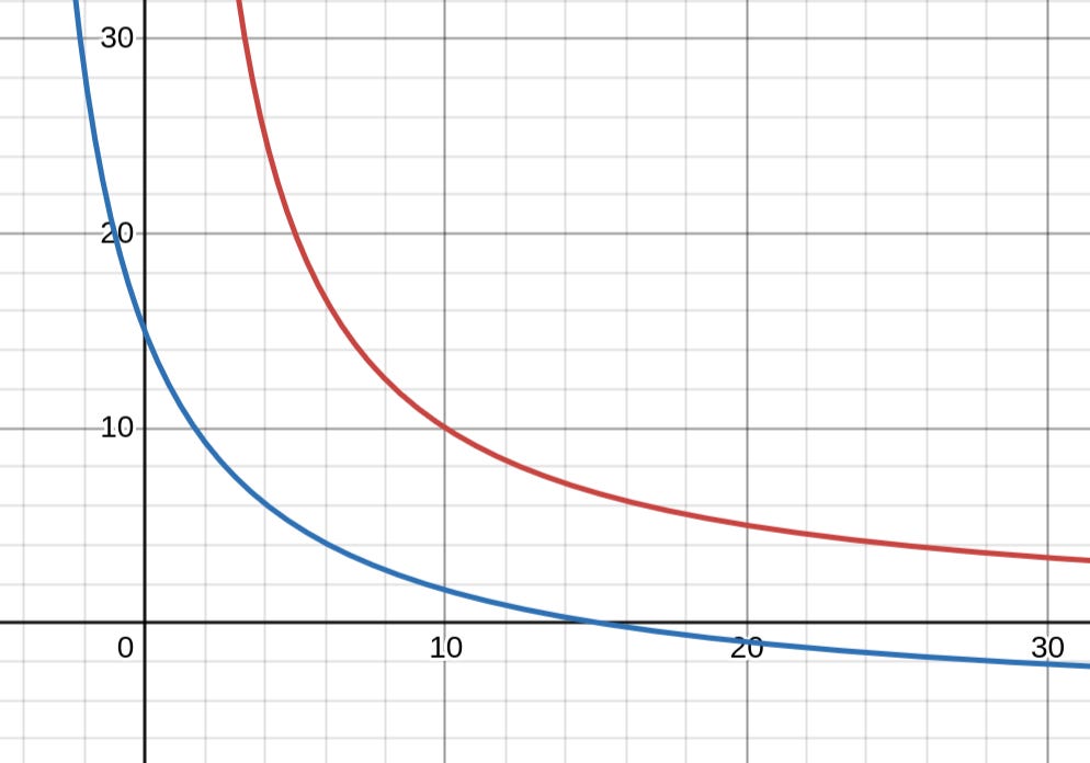
To visualize this, take an equation of the form:
This is equivalent to the equation:
Except shifted a units to the left, and b units down.
Here I’ve plotted the equation x*y=100 in red, and (x+5)(y+5)=100 in blue using the Desmos graphing calculator. This could represent a Uniswap V3 pool where the square of virtual liquidity equals 100, with offsets of 5 for each token to account for virtual liquidity.
The virtual reserves are not symmetric but the simple graph is sufficient to illustrate the concept. Per Equation 2.2, the x and y offsets depend on the prices associated with the liquidity position.
Convex Optimization
I prefer to base my calculation on real reserves because I can enforce price and amount contraints at either end of the liquidity range. This leads to the intuitive results that x=0 at price b, and y=0 at price a. Once we’ve hit zero, we are at the end of the liquidity range and have to shift to the next.
We will use CVXPY to model the swapping behavior of an imaginary 0.03% fee V3 pool with a single position of 100,000 liquidity between ticks 0 & 10. The current price of the pool is at tick 5.


